Table of Contents
Introduction to Hyperspectral Imaging
From single-banded monochrome imagery to spectrally dense hyperspectral imagery, capturing the spatial and spectral characteristics of a material has provided insight into a material’s structure, composition, and identity. This information can then be leveraged to elucidate the performance and quality characteristics of products in fields ranging from pharmaceuticals and biological imaging to plastics and agriculture. Single-banded monochrome systems, which offer the lowest density spectral information but high spatial sampling rates, give users high fidelity spatial characteristics but essentially no information on its spectral identity. Increasing the spectral sampling, but sacrificing some spatial information, red-green-blue (RGB) imagers capture color images of materials in easily interpretable bands for humans by employing Bayer filters. While RGB offers additional spectral information, materials under inspection must be well separated spectrally to properly distinguish one from another as the RGB bands of the Bayer filter are spectrally broad. Additionally, RGB bands overlap with one another, further distorting the true color of the materials under inspection.
Multispectral imagers are a step-up from RGB offering anywhere from 4-20 colors of interest. Some commercial products operate on a similar principle as RGB but with more spectral information and higher spectral tunability. There are plenty of multispectral systems available on the market and Surface Optics Corp. offers its own proprietary multispectral imagers leveraging our LightShift technology. While RGB is confined to the same 3 spectral bands, multispectral systems offer selectable spectral bands at different positions and widths catered to their intended application. However, since multispectral systems are often built for specific applications, they can fail when used in applications that experience materials with different spectral regions of interest as the system requires different filter trays, detectors, or optics to adapt the camera.
To better define the unique spectral signature of a material, hyperspectral imaging systems (HSI) have been developed. These systems have anywhere from twenty to hundreds or even thousands of color bands. Traditionally, a camera and spectrograph are configured in the traditional push broom geometry where a spatial axis of the camera is sacrificed for spectral definition, and one spatial axis is maintained. This results in the need for the camera or the object to be scanned across the field of view of the fore-optics to collect a full hyperspectral image cube. Surface Optics Corp. has a history of delivering hyperspectral imagers that leverage camera scanning image collection – SOC-710, SOC-760, and SOC-750 product lines. A unique advantage of the 710 product is its fully internal camera scanning feature that makes integration into advanced measurement workflows or imaging systems simple as no mechanical scanning of the camera or object need be considered. Instead, the user treats the whole system as a highly integrable component and simply mates the native C-mount of the SOC-710 to their optical system, i.e. a microscope or specialized imaging system, and they are immediately enabled to collect 3-D hyperspectral images.
Recently, SOC has developed an updated version of the SOC-710 product line, starting with the Visible-Near-Infrared (VNIR) camera scanning SOC-710 variant, the SOC-710 OmniCore. This product enables users looking for a turn-key solution to collect 4-D hyperspectral images immediately out of the box. For integrators, we are also excited to announce a non-scanning hyperspectral camera, SOC-710 HyCore, which enables hyperspectral image collection from a drone, in a roll-to-roll production line, or other object scanning measurement scenarios. Here we provide insight into the selection and comparison of hyperspectral imaging systems as well as a case study highlighting the integrability of the new 710-OmniCore into imaging systems.
Key Performance Characteristics of Hyperspectral Imaging Systems to Consider
There are many ways of representing a HSI’s performance and SOC strives to provide an accurate representation of our products’ specifications. For HSI’s, four parameters paint a good picture of a system’s performance: maximum signal-to-noise ratio (SNR), pixel size, frame rate, and spectral resolution. Here we provide a non-exhaustive overview of each characteristic, and a summary of how each one relates to real-world performance.
Maximum Signal-to-Noise
SNR is a critical parameter that informs us on how well the sensor collects desirable signals and distinguishes these signals from unwanted noise to produce actionable data. On a pixel-by-pixel basis, a camera can only attain a defined maximum SNR which is limited by the electrical performance of the camera. Specifically, the well depth (e–), dark current (e–/s), read noise (e–) and spectrally dependent quantum efficiency (unitless). If these values are known, one can calculate the maximum SNR ratio with the following formula:
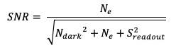
Where,
Here we assume the illumination is optimized and maximized, which in practice can be optimized but not maximized, however, allows us to compare sensor to sensor irrespective of the lighting conditions, which can vary drastically. A higher SNR means a sensor is better at collecting signals and rejecting noise. For cameras, SNR is influenced by many factors including the camera binning. Higher binning leads to higher SNR values. For example, a binning of 1×1 pixels may have an SNR of 100. Increasing the binning to 2×2 will double the potential SNR to 200 but at the cost of resolution, since a single pixel is essentially 4 combined pixels. It’s important to optimize binning settings for your application. If more signal and less resolution is desired, increasing binning is a great idea. However, if you are interested in the fine details, spectrally and spatially, keeping the binning at the lowest setting will provide the most density of information. For SOC’s new 710 VNIR products, a maximum SNR of 222 was calculated at a binning of 1×2 (spatial x spectral) which is comparable to competitors’ products.
Pixel Size
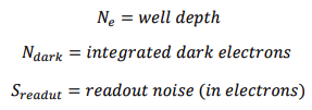
Pixel size is important for calculating the maximum SNR as well as the minimum resolvable object for the camera. For SNR, an increase in pixel size, assuming the pixels well depth scales as well, leads to a larger SNR as a larger area is exposed measuring more photons and therefore more signal. Binning can also be treated as increasing the exposed area and well depth by adding the signal collected by adjacent pixels, creating a super pixel. As an example, consider two cameras with the same hardware characteristics (well depth, dark current, readout noise) but camera 1 has pixel size of 5 microns and camera 2 has a pixel size of 10. Since camera 1 has pixels that are 4x less area than camera 2, we expect under identical acquisition settings that camera 1 will have a SNR 2x smaller than camera 2.
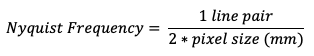
Although higher SNRs can be achieved with larger pixel sizes or through binning, all else being equal, there’s a tradeoff. As pixel size increases, the spatial and spectral resolution of an HSI deteriorates. This is due to a decrease in the optical sampling rate provided by the camera. Let’s look at the previous example again with 5- and 10-micron pixel sizes. Here, the Nyquist frequency, the theoretical limit of resolution expressed in line pairs per millimeter (lp/mm), is 100 lp/mm for the 5micron pixel camera and 50lp/mm for the 10micron pixel. A higher Nyquist frequency indicates an optical component can resolve finer details. In the case of HSIs this means higher potential spectral and spatial resolution if well matched with other optical components.
Frame Rate
Next, we consider frame rate which gives us details on how quickly the camera can collect and translate information. An HSI’s frame rate is limited by the electronics supporting the sensor as well as the computer the HSI is connected to. Assuming data transmission is not limiting, (i.e. using adequate connections from the computer to the camera) the frame rate will be limited by the camera electronics (sensor supporting electronics). Here, we can express the framerate for a full-frame integrate-then-read sensor with the following equation:
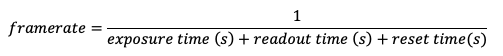
It’s important to note that at lower exposure times, readout and reset times dominate framerate. For example, the minimum exposure time for HyCore and OmniCore is 1 ms. However, the maximum full-frame framerate is 195 fps (~5.1 ms to collect a frame). Therefore, readout and reset time more than quintuple the amount of time required to read and digitize an image. The chart below shows an estimate of frame rate at different binnings (only in 1×N or N×1).
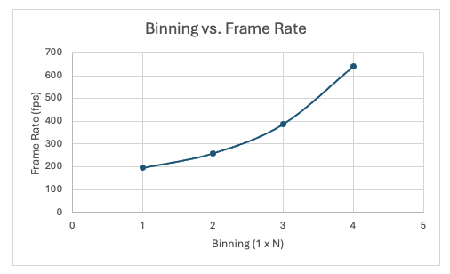
Figure 1. Plot showing calculated frame rates as binning is increased and the number of pixels read out decreases.
Spectral Resolution
Finally, we will consider spectral resolution. This performance characteristic is limited by both the sensor and connected spectrograph assembly. Since it was already mentioned that smaller sensor pixels produce higher spectral resolution, we will only consider spectrograph performance here. Without going into exhaustive detail about the spectrograph and its components, an important concept to understand is that a low-performance component in an optical system often has the greatest impact on overall system performance, as intuition would suggest. If the selected camera resolution exceeds the performance capability of the spectrograph, then the cost associated with that higher-performance camera becomes unnecessary. In the case of the SOC 710 HyCore and OmniCore products, the camera and spectrograph were designed so their performance is closely matched. This results in a best-in-class spectral resolution of 1.65 nm at a spectral binning of 0.
HyCore and OmniCore Performance Characterization
A full characterization of the new SOC-710 product was performed using standard light sources and resolution targets. Electronic performance characteristics are derived from the sensor and supporting electronics and were outlined previously in our discussion of frame rate and binning.
| Characteristic | Value |
| Spectral Bands | 784 |
| Spatial Bands | 1500 |
| Spectral Resolution | 1.65 nm |
| Max Frame Rate @ full frame | 195 fps |
| Pixel Size | 5.86 µm |
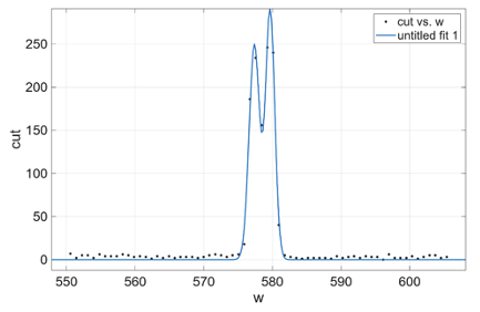
Spectral characteristics were also determined using standard spectral lamps from Oriel. Using mercury-argon gas lamps, spectral definition and calibration of the camera were performed with a default spectral binning of 1. A challenging feature for many hyperspectral imagers to resolve is the Hg-Ar lamp doublet around 580 nm. As shown below, the new SOC-710 product has no issue resolving these peaks.
It is important to note that these gas lines have spectral widths much smaller than the resolving power of the spectrograph used in HyCore. Therefore, HyCore can achieve spectral and spatial focusing down to the Nyquist frequency (2 pixels), resulting in a spectral resolution of 1.65 nm.
The density of spectral information offers users ease-of-mind during measurements, giving confidence that the true reflective properties of their materials are being collected.
Integration into Microscope Platform
To highlight potential applications for our SOC-710 OmniCore product, we integrated the camera into a simple, bright-field microscope. It’s important to note that a halogen lamp was used as the source, and we suggest you use one too. Halogen sources provide near-infrared (NIR) light (~800nm+) that standard LED sources do not. Below is a plot demonstrating the spectral output of a variety of sources as well as the sensitivity of the human eye for perspective. It’s clear that standard LED sources do not provide broadband spectral luminance and should be avoided. There are LED sources that extend into the NIR, but they can be cost prohibitive.
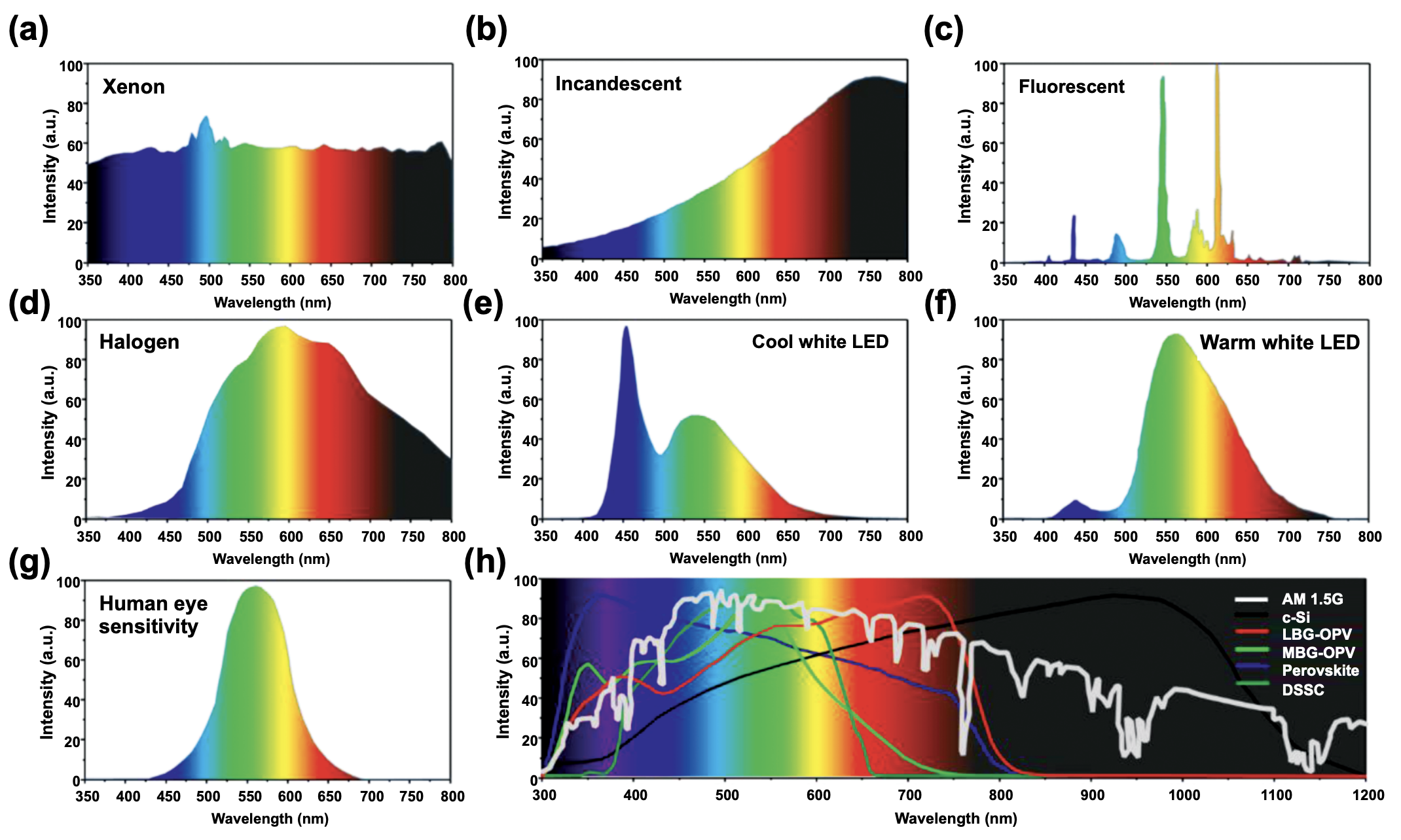
To highlight potential applications for our SOC-710 OmniCore product, we integrated the camera into a simple bright-field microscope. It’s important to note that a halogen lamp was used as the source, and we suggest you use one too. Halogen sources provide near-infrared (NIR) light (~800 nm+) that standard LED sources do not. Below is a plot demonstrating the spectral output of a variety of sources, as well as the sensitivity of the human eye for perspective. It’s clear that standard LED sources do not provide broadband spectral luminance and should be avoided. There are LED sources that extend into the NIR, but they can be cost prohibitive.
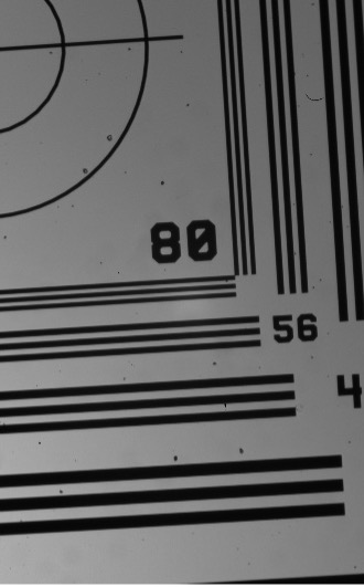
Hyperspectral images of an Air Force 1952 target were collected first to demonstrate the performance of the OmniCore-microscope integration. An RGB image generated from the data is shown below and an overlaid edge-spread and line-spread plots. With this data, the modulation transfer function (MTF) of the system can be calculated with a standard slanted edge analysis workflow. The MTF of an optical system indicates its ability to preserve object-side detail during the imaging process. The MTF of an optical system is often limited by specific optical components and here we attempt to determine the limiting component in our simple demonstration. For our sensor, with a pixel size of 5.86 µm, the maximum MTF that can be achieved is 85.3 lp/mm.
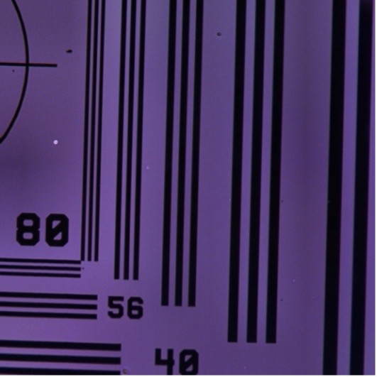
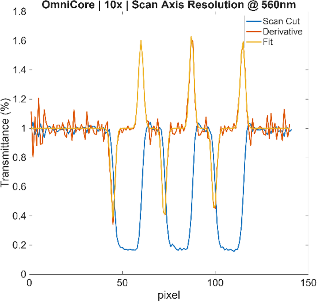
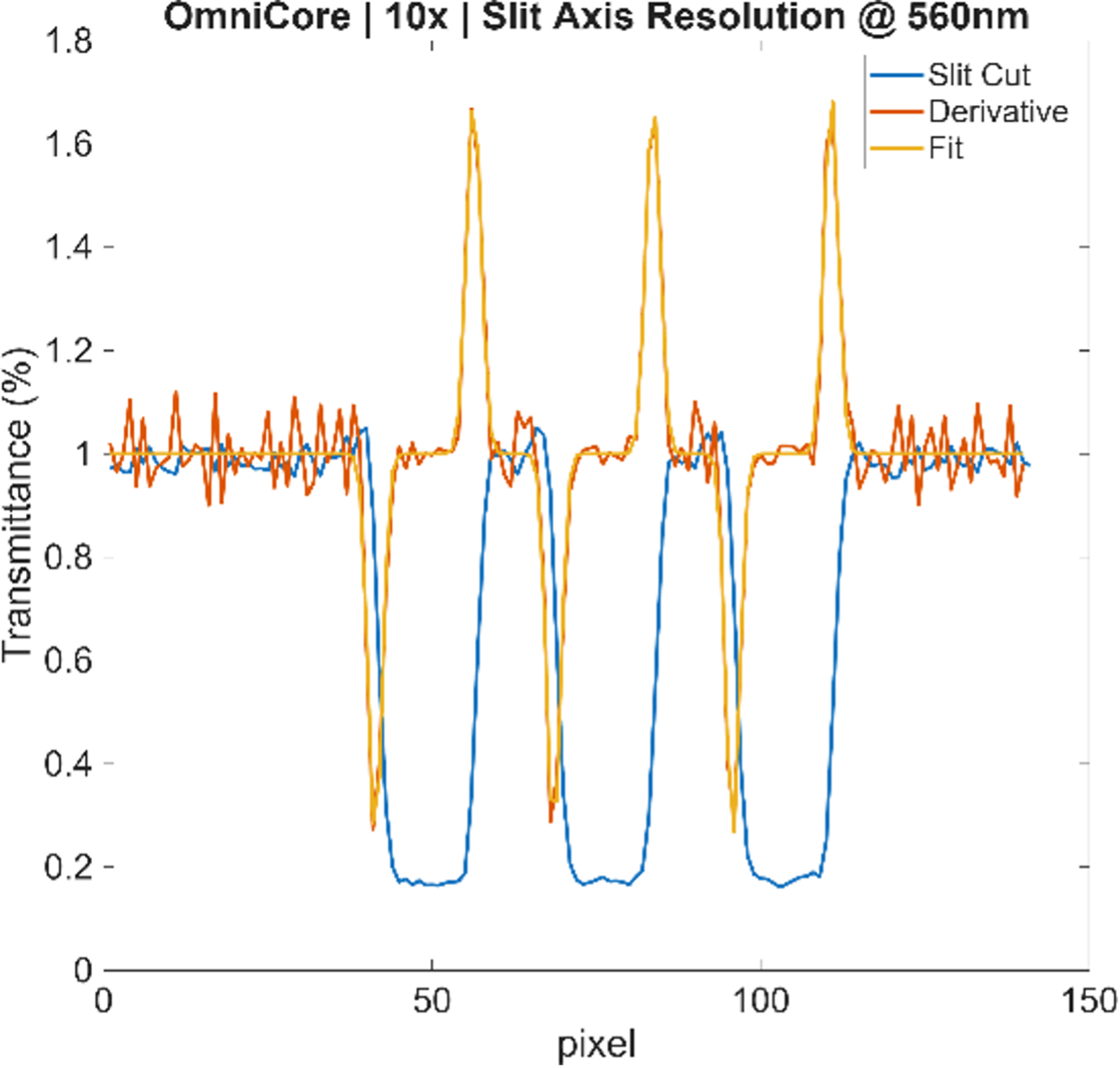
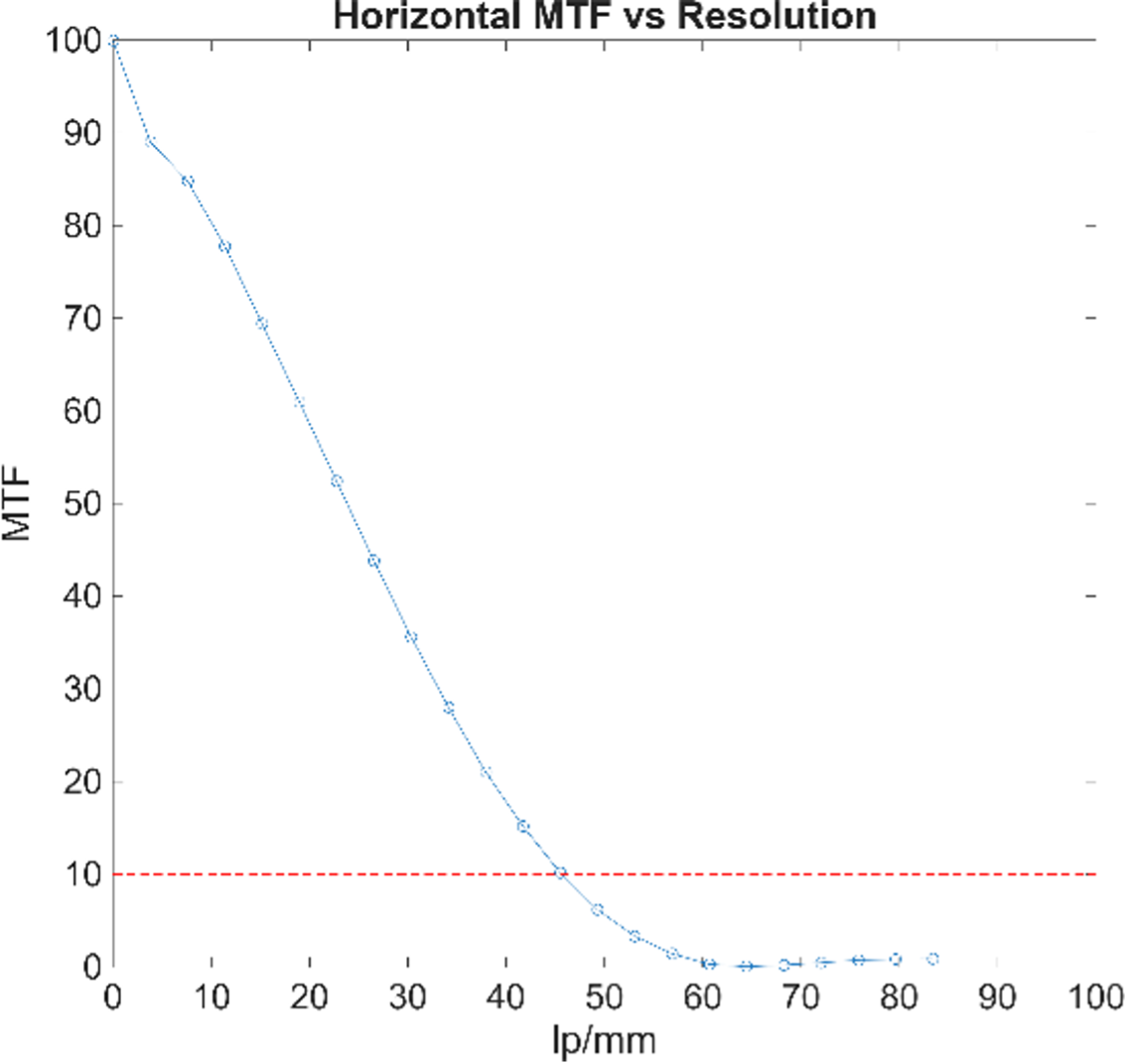

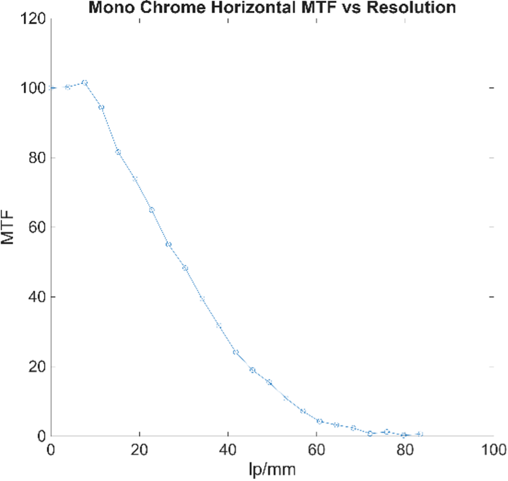
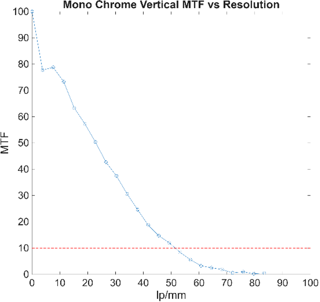
The plots above depict the horizontal and vertical MTF curves of the OmniCore and brightfield microscope integration at 10× magnification (Figures 8 and 9), as well as the horizontal and vertical MTF curves of the monochrome sensor (Figures 10 and 11) used in HyCore and OmniCore.
Figures 8 and 9 indicate there is minimal difference between optical performance in the vertical (slit axis) and horizontal (mechanical scan axis) directions, with both axes exhibiting 10% MTF values of approximately 45 lp/mm.
For a magnification of 10×, the resolution at an MTF of 10% is multiplied by 10 to determine the object-side resolution of the optical system, resulting in 450 lp/mm. This corresponds to a minimum resolvable feature size of approximately 1.1 µm for this demonstration.
These results highlight the mechanical stability of OmniCore and its high-performance camera-scanning image collection workflow.
When the MTF of the HSI is compared with that of the bare sensor (Figures 10 and 11), only a modest reduction in performance is observed. For the bare sensor in both axes, an MTF of 10% occurs at a resolution of approximately 52 lp/mm, resulting in an object-side resolution of 1 µm.
Therefore, only a small decrease in performance is observed when the spectrograph is added to the optical path. We also note that spatial resolution can be further improved through the use of higher-performance imaging components than those used in this simple demonstration.
Additionally, we are exploring how oversampling in the spatial and spectral axes may further increase resolution through super-resolution techniques.
Hyperspectral Microscopy of H&E-Stained Bone Tissue
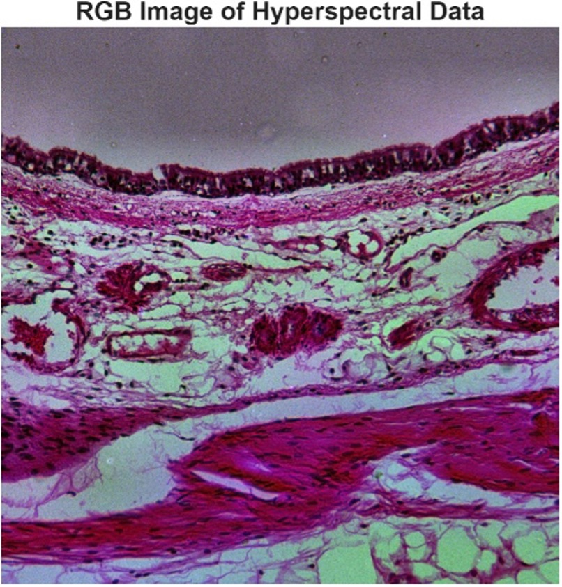
Beyond measuring the performance of OmniCore, hyperspectral images were collected using the same off-the-shelf microscope described previously. Hyperspectral images of a fixed, Hematoxylin and Eosin (H&E) stained mammal bone were collected. This staining procedure provides good contrasts between tissue and cellular structures. With this staining protocol, nuclei are stained as dark purple while cytoplasmic components are stained pink. The data was collected at the maximum irradiance of the imaged area, which was limited by the intensity of the quartz halogen lamp used. Exposure times for each scanned line were set at 200 ms for a total image collection time of ~5 mins. More powerful light sources can be used to reduce exposure times and total image acquisition times.
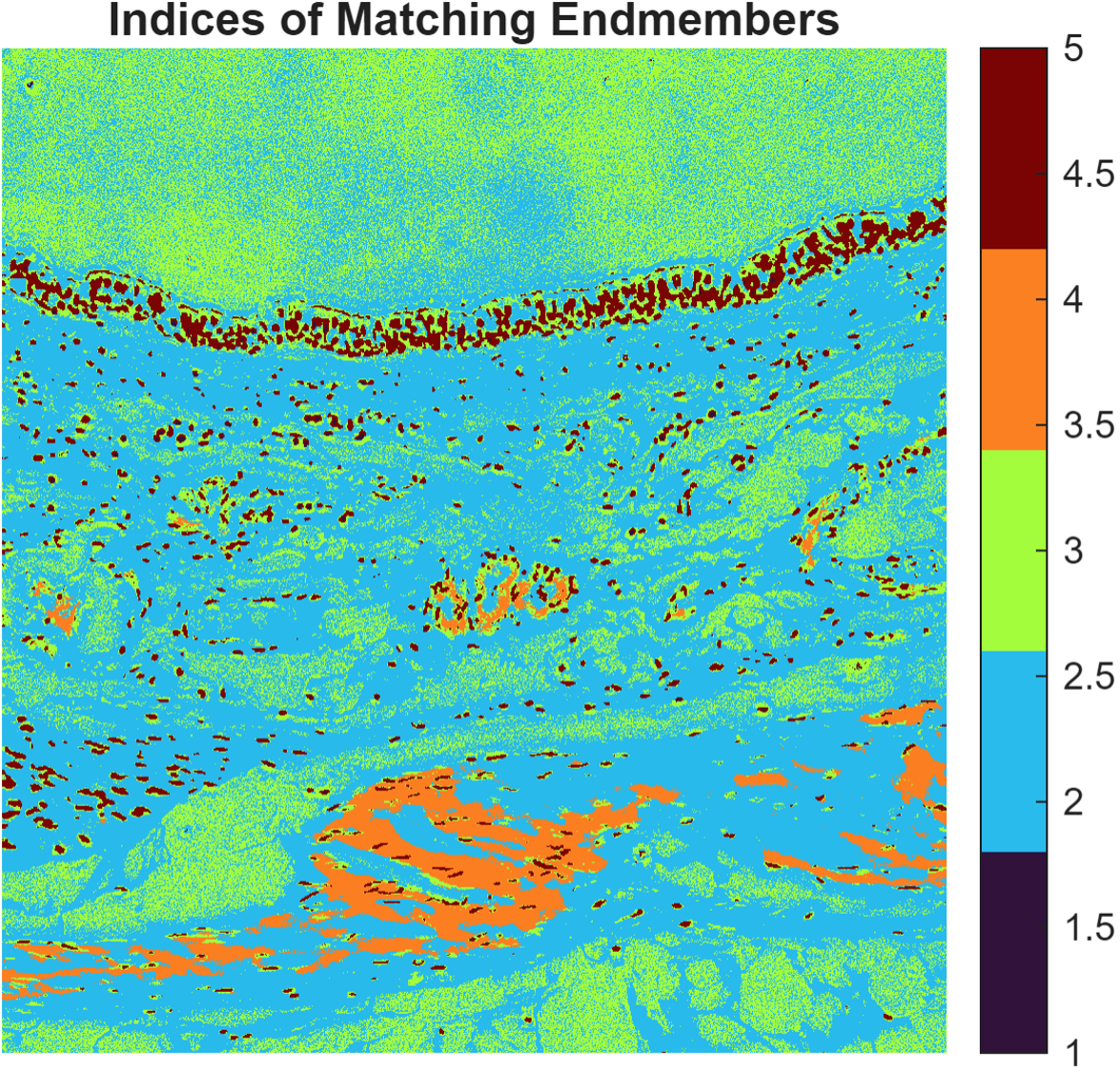
The 1500 x 1500 x 856 hypercube was first flat fielded by dividing the raw data by an image area of the microscope slide without any tissue. This corrects for intensity variations that exist over the field of view, increasing the performance of the target detection algorithm used later. An RGB image of the hyperspectral data is shown in Figure 12. After the image was flat fielded, the number of endmembers was determined with MatLab’s Hyperspectral Image Processing toolbox using the nfindr detection algorithm. This resulted in 5 unique spectra detected, Figure 14, which were used in a hybrid spectral information divergence (SID) and spectral angle mapper (SAM) target matching algorithm sidsam, which is included in the MatLab toolbox. Signature 1 is found within a few nuclei across the entire image. Signatures 2 and 3 are mapped as the pink tissue regions with spectral intensity and shape differences that may indicate unique structures. Signature 4 clearly tracks with nuclei detection which are easily seen in the RGB image. Examples for this data and data workflows can be used for applications such as high-throughput histopathology, spectral unmixing of multi-labeled slides, and other imaging applications that would benefit from additional color information.

Get a Quote for the 710 Series Hyperspectral Imaging System
VNIR hyperspectral imaging from 375–1025 nm. Trusted by researchers, integrators, and defense labs worldwide.
- Radiometrically calibrated in-lab
- SDK for C#, C++, and Python
- Microscope, lab & field compatible
- Complete hyperspectral imaging system